使用 Core API 进行矩阵逼近

#@title Licensed under the Apache License, Version 2.0 (the "License");
# you may not use this file except in compliance with the License.
# You may obtain a copy of the License at
#
# https://www.apache.org/licenses/LICENSE-2.0
#
# Unless required by applicable law or agreed to in writing, software
# distributed under the License is distributed on an "AS IS" BASIS,
# WITHOUT WARRANTIES OR CONDITIONS OF ANY KIND, either express or implied.
# See the License for the specific language governing permissions and
# limitations under the License.

使用 Core API 进行矩阵逼近#

在 TensorFlow.org 上查看

在 Google Colab 运行

在 GitHub 上查看源代码

下载笔记本

简介#

此笔记本使用 TensorFlow Core 低级 API 展示了 TensorFlow 作为高性能科学计算平台的能力。访问 Core API 概述以详细了解 TensorFlow Core 及其预期用例。

本教程探讨奇异值分解 (SVD) 技术及其在低秩逼近问题中的应用。SVD 用于分解实数或复数矩阵，并在数据科学中具有多种用例，例如图像压缩。本教程的图像来自 Google Brain 的 Imagen 项目。

安装#

import matplotlib
from matplotlib.image import imread
from matplotlib import pyplot as plt
import requests
# Preset Matplotlib figure sizes.
matplotlib.rcParams['figure.figsize'] = [16, 9]

import tensorflow as tf
print(tf.__version__)

SVD 基础知识#

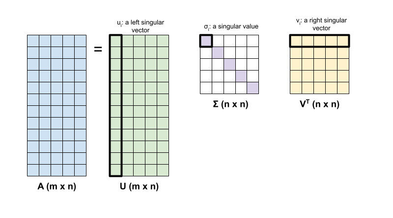
矩阵 $A$ 的奇异值分解由以下因式分解确定：

A = U Σ V^{T}

其中

$\underset{m \times n}{A}$ ：输入矩阵，其中 $m \geq n$
$\underset{m \times n}{U}$ ：正交矩阵， $U^{T} U = I$ ，包含各个列 $u_{i}$ ，表示 $A$ 的左奇异向量
$\underset{n \times n}{Σ}$ ：对角矩阵，包含各个对角条目 $σ_{i}$ ，表示 $A$ 的奇异值
$\underset{n \times n}{V^{T}}$ ：正交矩阵， $V^{T} V = I$ ，包含各个行 $v_{i}$ ，表示 $A$ 的右奇异向量

当 $Misplaced &$ 时， $U$ 和 $Σ$ 的维度均为 $(m \times m)$ ，而 $V^{T}$ 的维度为 $(m \times n)$ 。

TensorFlow 的线性代数软件包具有一个函数 tf.linalg.svd，可用于计算一个或多个矩阵的奇异值分解。首先，定义一个简单的矩阵并计算其 SVD 因式分解。

A = tf.random.uniform(shape=[40,30])
# Compute the SVD factorization
s, U, V = tf.linalg.svd(A)
# Define Sigma and V Transpose
S = tf.linalg.diag(s)
V_T = tf.transpose(V)
# Reconstruct the original matrix
A_svd = U@S@V_T
# Visualize 
plt.bar(range(len(s)), s);
plt.xlabel("Singular value rank")
plt.ylabel("Singular value")
plt.title("Bar graph of singular values");

tf.einsum 函数可用于根据 tf.linalg.svd 的输出直接计算矩阵重构。

A_svd = tf.einsum('s,us,vs -> uv',s,U,V)
print('\nReconstructed Matrix, A_svd', A_svd)

使用 SVD 进行低秩逼近#

矩阵的秩 $A$ 由其各列所跨越的向量空间的维度决定。SVD 可用于逼近具有较低秩的矩阵，这最终会降低存储矩阵表示的信息所需数据的维数。

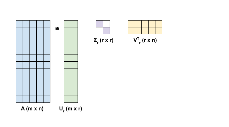
$A$ 在 SVD 中的秩 r 逼近由以下方程定义：

A_{r} = U_{r} Σ_{r} {V_{r}}^{T}

其中

$\underset{m \times r}{U_{r}}$ ：由 $U$ 的前 $r$ 列组成的矩阵
$\underset{r \times r}{Σ_{r}}$ ：由 $Σ$ 中的前 $r$ 个奇异值组成的对角矩阵
${\underset{r \times n}{V_{r}}}^{T}$ ：由 $V^{T}$ 的前 $r$ 行组成的矩阵

首先，编写一个函数来计算给定矩阵的秩 r 逼近。这种低秩逼近过程用于图像压缩；因此，计算每个逼近的物理数据大小也很有帮助。为简单起见，假设秩 r 逼近矩阵的数据大小等于计算逼近所需的元素总数。接下来，编写一个函数来呈现原始矩阵 $A$ 、其秩 r 逼近 $A_{r}$ 和误差矩阵 $| A - A_{r} |$ 。

def rank_r_approx(s, U, V, r, verbose=False):
  # Compute the matrices necessary for a rank-r approximation
  s_r, U_r, V_r = s[..., :r], U[..., :, :r], V[..., :, :r] # ... implies any number of extra batch axes
  # Compute the low-rank approximation and its size
  A_r = tf.einsum('...s,...us,...vs->...uv',s_r,U_r,V_r)
  A_r_size = tf.size(U_r) + tf.size(s_r) + tf.size(V_r)
  if verbose:
    print(f"Approximation Size: {A_r_size}")
  return A_r, A_r_size

def viz_approx(A, A_r):
  # Plot A, A_r, and A - A_r
  vmin, vmax = 0, tf.reduce_max(A)
  fig, ax = plt.subplots(1,3)
  mats = [A, A_r, abs(A - A_r)]
  titles = ['Original A', 'Approximated A_r', 'Error |A - A_r|']
  for i, (mat, title) in enumerate(zip(mats, titles)):
    ax[i].pcolormesh(mat, vmin=vmin, vmax=vmax)
    ax[i].set_title(title)
    ax[i].axis('off')

print(f"Original Size of A: {tf.size(A)}")
s, U, V = tf.linalg.svd(A)

# Rank-15 approximation
A_15, A_15_size = rank_r_approx(s, U, V, 15, verbose = True)
viz_approx(A, A_15)

# Rank-3 approximation
A_3, A_3_size = rank_r_approx(s, U, V, 3, verbose = True)
viz_approx(A, A_3)

正如预期的那样，使用较低的秩会得到不太准确的逼近。然而，这些低秩逼近的质量在现实世界的场景中通常足够好。另请注意，使用 SVD 进行低秩逼近的主要目标是减少数据的维数，而不是减少数据本身的磁盘空间。不过，随着输入矩阵的维度变高，许多低秩逼近也最终受益于缩减的数据大小。这种缩减的好处是该过程适用于图像压缩问题的原因。

图像加载#

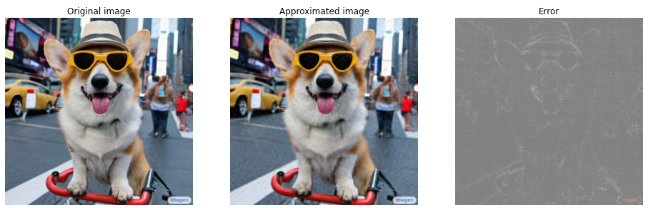
Imagen 首页上提供了以下图像。Imagen 是由 Google Research 的 Brain 团队开发的文本到图像扩散模型。AI 根据提示创建了这张图像：“一张柯基犬在时代广场骑自行车的照片。它戴着墨镜和沙滩帽。”多么酷啊！您还可以将下面的网址更改为任何 .jpg 链接以加载选择的自定义图像。

首先，读入并呈现图像。读取 JPEG 文件后，Matplotlib 会输出一个形状为 $(m \times n \times 3)$ 的矩阵 $I$ ，它表示一个二维图像，具有分别对应于红色、绿色和蓝色的 3 个颜色通道。

img_link = "https://imagen.research.google/main_gallery_images/a-photo-of-a-corgi-dog-riding-a-bike-in-times-square.jpg"
img_path = requests.get(img_link, stream=True).raw
I = imread(img_path, 0)
print("Input Image Shape:", I.shape)

def show_img(I):
  # Display the image in matplotlib
  img = plt.imshow(I)
  plt.axis('off')
  return

show_img(I)

图像压缩算法#

现在，使用 SVD 计算样本图像的低秩逼近。回想一下，图像的形状为 $(1024 \times 1024 \times 3)$ ，并且 SVD 理论仅适用于二维矩阵。这意味着必须将样本图像批处理为 3 个大小相等的矩阵，这些矩阵对应于 3 个颜色通道中的每一个。这可以通过将矩阵转置为形状 $(3 \times 1024 \times 1024)$ 来实现。为了清楚地呈现逼近误差，将图像的 RGB 值从 $[0, 255]$ 重新缩放到 $[0, 1]$ 。记得在呈现它们之前将逼近值裁剪到此区间内。tf.clip_by_value 函数对此十分有用。

def compress_image(I, r, verbose=False):
  # Compress an image with the SVD given a rank 
  I_size = tf.size(I)
  print(f"Original size of image: {I_size}")
  # Compute SVD of image
  I = tf.convert_to_tensor(I)/255
  I_batched = tf.transpose(I, [2, 0, 1]) # einops.rearrange(I, 'h w c -> c h w')
  s, U, V = tf.linalg.svd(I_batched)
  # Compute low-rank approximation of image across each RGB channel
  I_r, I_r_size = rank_r_approx(s, U, V, r)
  I_r = tf.transpose(I_r, [1, 2, 0]) # einops.rearrange(I_r, 'c h w -> h w c')
  I_r_prop = (I_r_size / I_size)
  if verbose:
    # Display compressed image and attributes
    print(f"Number of singular values used in compression: {r}")
    print(f"Compressed image size: {I_r_size}")
    print(f"Proportion of original size: {I_r_prop:.3f}")
    ax_1 = plt.subplot(1,2,1)
    show_img(tf.clip_by_value(I_r,0.,1.))
    ax_1.set_title("Approximated image")
    ax_2 = plt.subplot(1,2,2)
    show_img(tf.clip_by_value(0.5+abs(I-I_r),0.,1.))
    ax_2.set_title("Error")
  return I_r, I_r_prop

现在，计算以下秩的秩 r 逼近：100、50、10

I_100, I_100_prop = compress_image(I, 100, verbose=True)

I_50, I_50_prop = compress_image(I, 50, verbose=True)

I_10, I_10_prop = compress_image(I, 10, verbose=True)

评估逼近#

可以通过多种有趣的方法衡量有效性并更好地控制矩阵逼近。

压缩因子与秩#

对于上述每个逼近，观察数据大小如何随秩变化。

plt.figure(figsize=(11,6))
plt.plot([100, 50, 10], [I_100_prop, I_50_prop, I_10_prop])
plt.xlabel("Rank")
plt.ylabel("Proportion of original image size")
plt.title("Compression factor vs rank");

基于这张图，逼近图像的压缩因子与其秩之间存在线性关系。为了进一步探索这一点，回想一下，逼近矩阵 $A_{r}$ 的数据大小被定义为其计算所需的元素总数。下面的方程可用于找出压缩因子与秩之间的关系：

x = (m \times r) + r + (r \times n) = r \times (m + n + 1)

c = \frac{x}{y} = \frac{r \times (m + n + 1)}{m \times n}

其中

$x$ ： $A_{r}$ 的大小
$y$ ： $A$ 的大小
$c = \frac{x}{y}$ ：压缩因子
$r$ ：逼近的秩
$m$ 和 $n$ ： $A$ 的行维度和列维度

为了找到将图像压缩到所需因子 $c$ 所需的秩 $r$ ，可以重新排列上述方程以求解 $r$ ：

r = ⌊ \frac{c \times m \times n}{m + n + 1} ⌋

请注意，此公式与颜色通道维度无关，因为各个 RGB 逼近不会相互影响。现在，编写一个函数来压缩给定所需压缩因子的输入图像。

def compress_image_with_factor(I, compression_factor, verbose=False):
  # Returns a compressed image based on a desired compression factor
  m,n,o = I.shape
  r = int((compression_factor * m * n)/(m + n + 1))
  I_r, I_r_prop = compress_image(I, r, verbose=verbose)
  return I_r

将图像压缩到其原始大小的 15%。

compression_factor = 0.15
I_r_img = compress_image_with_factor(I, compression_factor, verbose=True)

奇异值的累积和#

奇异值的累积总和可作为秩 r 逼近捕获的能量量的有用指标。呈现样本图像中奇异值的 RGB 平均累积比例。tf.cumsum 函数对此十分有用。

def viz_energy(I):
  # Visualize the energy captured based on rank
  # Computing SVD
  I = tf.convert_to_tensor(I)/255
  I_batched = tf.transpose(I, [2, 0, 1]) 
  s, U, V = tf.linalg.svd(I_batched)
  # Plotting average proportion across RGB channels 
  props_rgb = tf.map_fn(lambda x: tf.cumsum(x)/tf.reduce_sum(x), s)
  props_rgb_mean = tf.reduce_mean(props_rgb, axis=0)
  plt.figure(figsize=(11,6))
  plt.plot(range(len(I)), props_rgb_mean, color='k')
  plt.xlabel("Rank / singular value number")
  plt.ylabel("Cumulative proportion of singular values")
  plt.title("RGB-averaged proportion of energy captured by the first 'r' singular values")

viz_energy(I)

看起来这个图像中超过 90% 的能量是在前 100 个奇异值中捕获的。现在，编写一个函数来压缩给定所需能量保留因子的输入图像。

def compress_image_with_energy(I, energy_factor, verbose=False):
  # Returns a compressed image based on a desired energy factor
  # Computing SVD
  I_rescaled = tf.convert_to_tensor(I)/255
  I_batched = tf.transpose(I_rescaled, [2, 0, 1]) 
  s, U, V = tf.linalg.svd(I_batched)
  # Extracting singular values
  props_rgb = tf.map_fn(lambda x: tf.cumsum(x)/tf.reduce_sum(x), s)
  props_rgb_mean = tf.reduce_mean(props_rgb, axis=0)
  # Find closest r that corresponds to the energy factor
  r = tf.argmin(tf.abs(props_rgb_mean - energy_factor)) + 1
  actual_ef = props_rgb_mean[r]
  I_r, I_r_prop = compress_image(I, r, verbose=verbose)
  print(f"Proportion of energy captured by the first {r} singular values: {actual_ef:.3f}")
  return I_r

压缩图像以保留 75% 的能量。

energy_factor = 0.75
I_r_img = compress_image_with_energy(I, energy_factor, verbose=True)

误差和奇异值#

逼近误差与奇异值之间也存在一个有趣的关系。事实证明，逼近的平方 Frobenius 范数等于其被省略的奇异值的平方和：

{| | A - A_{r} | |}^{2} = \sum_{i = r + 1}^{R} σ_{i}^{2}

使用本教程开头的示例矩阵的秩 10 逼近来测试这种关系。

s, U, V = tf.linalg.svd(A)
A_10, A_10_size = rank_r_approx(s, U, V, 10)
squared_norm = tf.norm(A - A_10)**2
s_squared_sum = tf.reduce_sum(s[10:]**2)
print(f"Squared Frobenius norm: {squared_norm:.3f}")
print(f"Sum of squared singular values left out: {s_squared_sum:.3f}")

结论#

此笔记本介绍了使用 TensorFlow 实现奇异值分解并将其应用于编写图像压缩算法的过程。下面是一些可能有所帮助的提示：

TensorFlow Core API 可用于各种高性能科学计算用例。
要详细了解 TensorFlow 线性代数功能，请访问 linalg 模块的文档。
SVD 也可应用于构建推荐系统。

有关使用 TensorFlow Core API 的更多示例，请查阅指南。如果您想详细了解如何加载和准备数据，请参阅有关图像数据加载或 CSV 数据加载的教程。