探索洛伦兹微分方程系统

在这个笔记本中，我们探索了洛伦兹微分方程系统：

\[ \begin{aligned} \dot{x} & = \sigma(y-x) \\ \dot{y} & = \rho x - y - xz \\ \dot{z} & = -\beta z + xy \end{aligned} \]

这是非线性微分方程中的一个经典系统。随着参数（\(\sigma\)，\(beta\)，\(\rho\)）的变化，它展现出一系列不同的行为。

首先，我们从 IPython、NumPy、Matplotlib 和 SciPy 中导入所需的库。

%matplotlib inline

from ipywidgets import interact, interactive
from IPython.display import clear_output, display, HTML

import numpy as np
from scipy import integrate

from matplotlib import pyplot as plt
from mpl_toolkits.mplot3d import Axes3D
from matplotlib.colors import cnames
from matplotlib import animation

计算轨迹并绘制结果

我们定义了一个函数，可以数值地积分微分方程，然后绘制解决方案。这个函数有控制微分方程参数（\(\sigma\)，\(\beta\)，\(\rho\)）的参数，数值积分（N，max_time）以及可视化（angle）。

def solve_lorenz(N=10, angle=0.0, max_time=4.0, sigma=10.0, beta=8./3, rho=28.0):

    fig = plt.figure()
    ax = fig.add_axes([0, 0, 1, 1], projection='3d')
    ax.axis('off')

    # prepare the axes limits
    ax.set_xlim((-25, 25))
    ax.set_ylim((-35, 35))
    ax.set_zlim((5, 55))
    
    def lorenz_deriv(x_y_z, t0, sigma=sigma, beta=beta, rho=rho):
        """Compute the time-derivative of a Lorenz system."""
        x, y, z = x_y_z
        return [sigma * (y - x), x * (rho - z) - y, x * y - beta * z]

    # Choose random starting points, uniformly distributed from -15 to 15
    np.random.seed(1)
    x0 = -15 + 30 * np.random.random((N, 3))

    # Solve for the trajectories
    t = np.linspace(0, max_time, int(250*max_time))
    x_t = np.asarray([integrate.odeint(lorenz_deriv, x0i, t)
                      for x0i in x0])
    
    # choose a different color for each trajectory
    colors = plt.cm.viridis(np.linspace(0, 1, N))

    for i in range(N):
        x, y, z = x_t[i,:,:].T
        lines = ax.plot(x, y, z, '-', c=colors[i])
        plt.setp(lines, linewidth=2)

    ax.view_init(30, angle)
    plt.show()

    return t, x_t

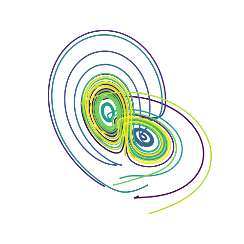
让我们调用一次函数来查看解决方案。对于这组参数，我们看到轨迹围绕两个点旋转，这两个点称为吸引子(attractors)。

t, x_t = solve_lorenz(angle=0, N=10)

使用 IPython 的 interactive 函数，我们可以探索当我们改变各种参数时轨迹的行为。

w = interactive(solve_lorenz, angle=(0.,360.), max_time=(0.1, 4.0), 
                N=(0,50), sigma=(0.0,50.0), rho=(0.0,50.0))
display(w)

由 interactive 返回的对象是一个 Widget 对象，它具有包含当前结果和参数的属性：

t, x_t = w.result

w.kwargs

{'N': 10,
 'angle': 0.0,
 'max_time': 4.0,
 'sigma': 10.0,
 'beta': 2.6666666666666665,
 'rho': 28.0}

在与系统交互之后，我们可以取结果并进行进一步的计算。在这个例子中，我们计算了 (x)、(y) 和 (z) 的平均位置。

xyz_avg = x_t.mean(axis=1)

xyz_avg.shape

(10, 3)

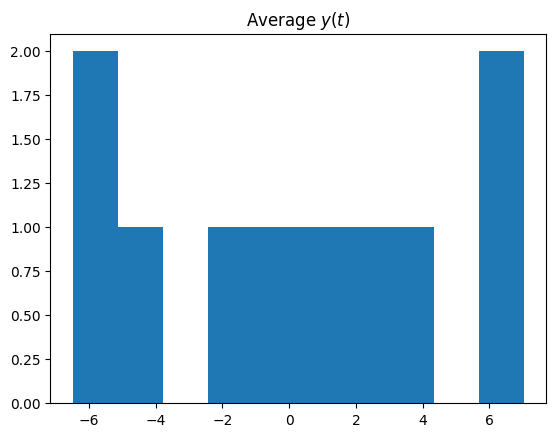
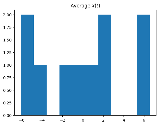
创建平均位置（跨不同轨迹）的直方图表明，平均而言，轨迹围绕吸引子旋转。

plt.hist(xyz_avg[:,0])
plt.title('Average $x(t)$');

plt.hist(xyz_avg[:,1])
plt.title('Average $y(t)$');